1. Introduction
This project presents an intelligent waste classification system that uses Convolutional Neural Networks (CNNs) to automatically sort waste into six predefined groups. It demonstrates how deep learning can be effectively applied in environmental management and automated recycling, improving classification accuracy while reducing human involvement in waste processing operations.
The model has been trained on the TrashNet dataset, which contains 2,527 labeled images across six waste categories: cardboard, glass, metal, paper, plastic, and general trash. The system processes individual images and delivers classification predictions along with their corresponding confidence levels.
Core Features:
- Classification across six predefined waste categories
- Instant predictions for individual image inputs
- Display of confidence probabilities for each prediction
- Visual presentation of classification results
- Comprehensive evaluation and performance reporting
2. Methodology / Approach
2.1 Architecture Overview
The project employs a custom Convolutional Neural Network with the following design:
Network Structure:
- Three convolutional blocks, each containing Conv2D layers followed by MaxPooling
- Conv2D Layer 1: 32 filters with 3×3 kernels → MaxPooling (2×2)
- Conv2D Layer 2: 64 filters with 3×3 kernels → MaxPooling (2×2)
- Conv2D Layer 3: 32 filters with 3×3 kernels → MaxPooling (2×2)
- Flattening layer converting spatial features to 1D vectors
- Two dense layers (64 and 32 units) with ReLU activation and dropout regularization (0.2)
- Output layer: 6 units with softmax activation for multi-class classification
Total Parameters: 1,645,830 trainable parameters
2.2 Data Preparation Strategy
All images are resized to 224×224 pixels with RGB channels (3-channel input). The dataset employs a 90-10 train-validation split. Data augmentation techniques applied to training data include:
- Horizontal and vertical flipping
- Shear and zoom transformations
- Width and height shifts (10% range)
- Pixel value rescaling to [0,1] range
2.3 Training Configuration
Optimizer: Adam
Loss Function: Categorical Cross-Entropy
Evaluation Metrics: Accuracy, Precision, Recall
Callbacks: Early stopping (patience=50) and model checkpoint saving
Training Duration: 50 epochs with early stopping
3. Mathematical Framework
3.1 Convolutional Operation
The convolutional layer applies a set of learnable filters to extract features from the input:
$$\mathbf{Y}_{i,j} = \sigma\left(\sum_{m=0}^{k-1} \sum_{n=0}^{k-1} \mathbf{W}_{m,n} \cdot \mathbf{X}_{i+m, j+n} + b\right)$$
where:
- $\mathbf{Y}_{i,j}$ = output feature map at position $(i, j)$
- $\mathbf{W}$ = learnable filter weights (kernel size $k \times k$)
- $\mathbf{X}$ = input feature map
- $b$ = bias term
- $\sigma$ = activation function (ReLU)
3.2 Max Pooling Operation
Reduces spatial dimensions while retaining the most prominent features:
$$\mathbf{P}_{i,j} = \max_{m,n \in \text{pool}} \mathbf{Y}_{i \cdot s + m, j \cdot s + n}$$
where:
- $\mathbf{P}_{i,j}$ = pooled output at position $(i, j)$
- $s$ = stride (typically 2 for 2×2 pooling)
- pool = pooling window size (2×2 in this architecture)
3.3 Fully Connected Layer
After flattening, dense layers perform classification:
$$\mathbf{z} = \mathbf{W} \cdot \mathbf{x} + \mathbf{b}$$
$$\mathbf{a} = \sigma(\mathbf{z})$$
where:
- $\mathbf{x}$ = flattened feature vector
- $\mathbf{W}$ = weight matrix
- $\mathbf{b}$ = bias vector
- $\sigma$ = ReLU activation (hidden layers) or softmax (output layer)
3.4 Dropout Regularization
Randomly drops neurons during training to prevent overfitting:
$$\mathbf{h}_{\text{dropout}} = \mathbf{h} \odot \mathbf{m}$$
where:
- $\mathbf{h}$ = layer output
- $\mathbf{m}$ = binary mask (0 or 1) with dropout probability $p = 0.2$
- $\odot$ = element-wise multiplication
3.5 Softmax Activation
Converts logits to probability distribution for multi-class classification:
$$p_i = \frac{e^{z_i}}{\sum_{j=1}^{C} e^{z_j}}$$
where:
- $p_i$ = probability for class $i$
- $z_i$ = logit (raw output) for class $i$
- $C = 6$ = number of classes (cardboard, glass, metal, paper, plastic, trash)
3.6 Loss Function
Categorical Cross-Entropy measures the difference between predicted and true distributions:
$$\mathcal{L} = -\sum_{i=1}^{N} \sum_{c=1}^{C} y_{ic} \cdot \log(p_{ic})$$
where:
- $N$ = batch size
- $C = 6$ = number of classes
- $y_{ic}$ = true label (1 if sample $i$ belongs to class $c$, 0 otherwise)
- $p_{ic}$ = predicted probability for sample $i$ and class $c$
3.7 Performance Metrics
Accuracy:
$$\text{Accuracy} = \frac{\text{Number of Correct Predictions}}{\text{Total Number of Predictions}}$$
Precision (for class $c$):
$$\text{Precision}_c = \frac{TP_c}{TP_c + FP_c}$$
Recall (for class $c$):
$$\text{Recall}_c = \frac{TP_c}{TP_c + FN_c}$$
F1-Score (for class $c$):
$$F1_c = 2 \times \frac{\text{Precision}_c \times \text{Recall}_c}{\text{Precision}_c + \text{Recall}_c}$$
where:
- $TP_c$ = True Positives for class $c$
- $FP_c$ = False Positives for class $c$
- $FN_c$ = False Negatives for class $c$
3.8 Data Augmentation Transformations
Horizontal/Vertical Flip:
$$\mathbf{X}_{\text{flip}} = \mathbf{F} \cdot \mathbf{X}$$
where $\mathbf{F}$ is a flipping transformation matrix.
Rotation:
$$\mathbf{X}_{\text{rot}} = \mathbf{R}(\theta) \cdot \mathbf{X}$$
where $\mathbf{R}(\theta)$ is a rotation matrix with angle $\theta$.
Zoom/Shear:
$$\mathbf{X}_{\text{transform}} = \mathbf{T} \cdot \mathbf{X}$$
where $\mathbf{T}$ represents zoom or shear transformation.
Normalization:
$$\mathbf{X}_{\text{norm}} = \frac{\mathbf{X}}{255}, \quad \mathbf{X} \in [0, 255] \Rightarrow \mathbf{X}_{\text{norm}} \in [0, 1]$$
4. Dataset
Source: TrashNet (Stanford University)
Total Images: 2,527
Classes: 6
Class Distribution:
- Glass: 501 images
- Paper: 594 images
- Cardboard: 403 images
- Plastic: 482 images
- Metal: 410 images
- Trash: 137 images
Image Specifications: 512×384 pixels, RGB channels, photographed on white board with natural or room lighting
5. Requirements
requirements.txt
numpy>=1.19.0
pandas>=1.0.0
seaborn>=0.11.0
matplotlib>=3.3.0
plotly>=5.0.0
scikit-learn>=0.24.0
imutils>=0.5.0
tensorflow>=2.6.0
opencv-python>=4.5.0
6. Installation & Configuration
6.1 Environment Setup
# Clone the repository
git clone https://github.com/kemalkilicaslan/Garbage-Classification-with-Convolutional-Neural-Network-CNN.git
cd Garbage-Classification-with-Convolutional-Neural-Network-CNN

# Install dependencies
pip install -r requirements.txt
6.2 Project Structure
Garbage-Classification-with-CNN
├── Garbage-Classification-with-CNN.ipynb
├── README.md
├── requirements.txt
├── LICENSE
└── mymodel.keras
6.3 Required Setup
- Google Colab notebook with GPU acceleration (recommended)
- Sufficient storage for dataset (~500 MB)
- Trained model file:
mymodel.keras - Dataset mounted from Google Drive
7. Usage / How to Run
7.1 Training the Model
from google.colab import drive
drive.mount('/content/drive')

# Load and preprocess data
x, labels = load_datasets('/path/to/dataset')

# Create and train model
model = Sequential()
# [Layer definitions...]
model.compile(optimizer='adam', loss='categorical_crossentropy',
              metrics=[Precision(), Recall(), 'acc'])
history = model.fit(train_generator, epochs=50, validation_data=test_generator)
7.2 Making Predictions
# Single image prediction
img, predictions, predicted_class = model_testing('/path/to/image.jpg')
predicted_label = waste_labels[predicted_class]
confidence = np.max(predictions[0])
7.3 Batch Prediction on Random Samples
predict_random_samples(model, dir_path, num_classes=6)8. Application / Results
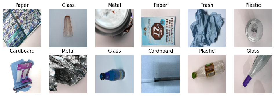
8.1 Dataset Visualization
Example images from the TrashNet dataset showing various waste categories used for training:
8.2 Model Performance
Test Set Metrics:
- Accuracy: 62.2%
- Precision: 76.7%
- Recall: 49.8%
- Loss: 1.0007
8.3 Per-Class Performance
| Class | Precision | Recall | F1-Score | Support |
|---|---|---|---|---|
| Cardboard | 0.95 | 0.50 | 0.66 | 40 |
| Glass | 0.56 | 0.70 | 0.62 | 50 |
| Metal | 0.50 | 0.66 | 0.57 | 41 |
| Paper | 0.74 | 0.93 | 0.83 | 59 |
| Plastic | 0.50 | 0.29 | 0.37 | 48 |
| Trash | 0.45 | 0.38 | 0.42 | 13 |
8.4 Training History
The following visualization displays the model's convergence behavior over 50 epochs, showing both training and validation loss, as well as accuracy metrics:

8.5 Confusion Matrix
The confusion matrix reveals classification patterns and misclassification tendencies across waste categories:

8.6 Sample Predictions
Real-world predictions on random test samples demonstrate model performance across all categories:

Prediction Examples:
- Cardboard: 99.90% confidence ✓
- Glass: 52.99% confidence ✓
- Plastic: 85.52% confidence ✓
- Paper: 44.38% confidence ✓
- Metal: 38.89% confidence ✓
9. Tech Stack
9.1 Core Technologies
- Programming Language: Python 3.6+
- Deep Learning Framework: TensorFlow/Keras 2.6+
- Computer Vision: OpenCV 4.5+
- Scientific Computing: NumPy 1.19+
9.2 Libraries & Dependencies
| Library | Version | Purpose |
|---|---|---|
| TensorFlow/Keras | 2.6+ | Deep learning framework for CNN |
| OpenCV | 4.5+ | Image processing and manipulation |
| NumPy | 1.19+ | Numerical computations and array operations |
| Scikit-learn | 0.24+ | Metrics and utilities |
| Matplotlib/Plotly | 3.3+/5.0+ | Data visualization |
9.3 Development Environment
- Google Colab with GPU acceleration
- Jupyter Notebook
- Google Drive for dataset storage
10. License
This project is licensed under the Creative Commons Attribution-NonCommercial-NoDerivatives 4.0 International (CC BY-NC-ND 4.0).
11. References
- Yang, M., & Thung, G. (2016). Classification of Trash for Recyclability Status. Stanford University CS229 Project Report.
- Krizhevsky, A., Sutskever, I., & Hinton, G. E. (2012). ImageNet Classification with Deep Convolutional Networks. Advances in Neural Information Processing Systems (NIPS), 25.
- TensorFlow Keras API Reference Documentation.
- OpenCV Image Processing Tutorials Documentation.
Acknowledgments
This project uses the TrashNet dataset created by Stanford University students Mindy Yang and Gary Thung. Special thanks to the TensorFlow and OpenCV communities for providing excellent deep learning and computer vision tools. The dataset was prepared for recyclability classification research and is used here for educational purposes.
Note: This project is intended for educational and research purposes. The model's performance (62.2% accuracy) demonstrates the practical challenges of real-world waste classification and suggests opportunities for improvement through enhanced training data, data augmentation, and transfer learning approaches such as fine-tuning pre-trained models (ResNet, MobileNet). When deploying waste classification systems in production environments, consider using larger datasets, advanced architectures, and regular model retraining to maintain accuracy.